Partitioned primary index or PPI is used for physically splitting the table into a series of subtables. With the proper use of Partition primary Index we can save queries from time consuming full table scan. Instead of scanning full table, only one particular partition is accessed.
Follow the example below to get the insight of PPI –
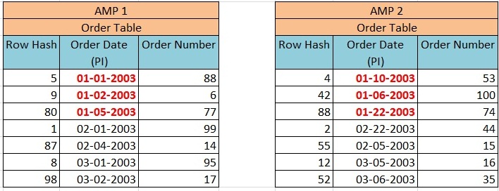
We have an order table (ORDER_TABLE) having two columns – Order_Date and Order_Number, in which PI is defined on Order_Date. The primary Index (Order_Date) was hashed and rows were distributed to the proper AMP based on Row Hash Value then sorted by the Row ID. The distribution of rows will take place as explained in the image below –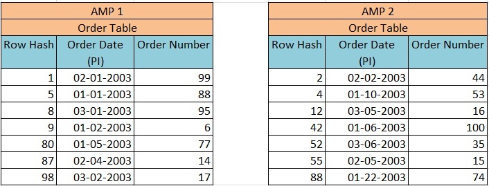
Now when we execute Query –
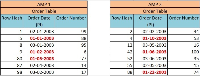
Select * from Order_Table where Order_Date between 1-1-2003 and 1-31-2003;
This query will result in a full table scan despite of Order_Date being PI.
Now we have defined PPI on the column Order_date. The primary Index (Order_Date) was hashed and rows were distributed to the proper AMP based on Row Hash Value then sorted by the Order_Date and not by Row ID. The distribution of rows will take place as explained in the image below –
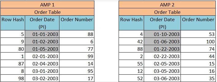
Now when we execute Query –
Select * from Order_Table where Order_Date between 1-1-2003 and 1-31-2003;
This query will not result in a full table scan because all the January orders are kept together in their partition.
Partitions are usually defined based on Range or Case as follows.
Partition by CASE
CREATE TABLE ORDER_Table (
ORDER_ID integer NOT NULL,
CUST_ID integer NOT NULL,
ORDER_DATE date ,
ORDER_AMOUNT integer
)
PRIMARY INDEX (CUST_ID)
PARTITION BY case_n (
ORDER_AMOUNT < 10000 ,
ORDER_AMOUNT < 20000 ,
ORDER_AMOUNT < 30000,
NO CASE OR UNKNOWN ) ;
Partition by RANGE
CREATE TABLE ORDER_Table
(
ORDER_ID integer NOT NULL,
CUST_ID integer NOT NULL,
ORDER_DATE date ,
ORDER_AMOUNT integer
)
PRIMARY INDEX (CUST_ID)
PARTITION BY range_n (
ORDER_DATE BETWEEN date ‘2012-01-01’ and ‘2012-12-31’ Each interval ‘1’ Month,
NO range OR UNKNOWN ) ;
If we use NO RANGE or NO CASE – then all values not in this range will be in a single partition.
If we specify UNKNOWN, then all null values will be placed in this partition